Using R for Biomedical Statistics
Biomedical statistics
This booklet tells you how to use the R software to carry out some simple analyses that are common in biomedical statistics. In particular, the focus is on cohort and case-control studies that aim to test whether particular factors are associated with disease, randomised trials, and meta-analysis.
This booklet assumes that the reader has some basic knowledge of biomedical statistics, and the principal focus of the booklet is not to explain biomedical statistics analyses, but rather to explain how to carry out these analyses using R.
If you are new to biomedical statistics, and want to learn more about any of the concepts presented here, I would highly recommend the Open University book “Medical Statistics” (product code M249/01), available from from the Open University Shop.
There is a pdf version of this booklet available at https://media.readthedocs.org/pdf/a-little-book-of-r-for-biomedical-statistics/latest/a-little-book-of-r-for-biomedical-statistics.pdf.
If you like this booklet, you may also like to check out my booklet on using R for time series analysis, http://a-little-book-of-r-for-time-series.readthedocs.org/ and my booklet on using R for multivariate analysis, http://little-book-of-r-for-multivariate-analysis.readthedocs.org/.
Calculating Relative Risks for a Cohort Study
One very common type of data set in biomedical statistics is a cohort study, where you have information on people who were exposed to some treatment or environment (for example, people who took a certain drug, or people who smoke) and also on whether the same people have a particular disease or not. Your data set would look something like this:
| Disease | Control | |
|---|---|---|
| Exposed | 156 | 9421 |
| Unexposed | 1531 | 14797 |
You can enter the data in R by typing:
> mymatrix <- matrix(c(156,9421,1531,14797),nrow=2,byrow=TRUE)
> colnames(mymatrix) <- c("Disease","Control")
> rownames(mymatrix) <- c("Exposed","Unexposed")
> print(mymatrix)
           Disease Control
Exposed       156    9421
Unexposed    1531   14797
The relative risk of having the disease given exposure is the probability of having the disease for people who were exposed to the treatment or environmental factor, divided by the probability of having the disease for people who were not exposed to that treatment or environmental factor.
You can calculate the relative risk of having the disease given exposure in R, by using a function calcRelativeRisk(). To be able to use this function, just copy the following code and paste it into R:
> calcRelativeRisk <- function(mymatrix,alpha=0.05,referencerow=2)
  {
     numrow <- nrow(mymatrix)
     myrownames <- rownames(mymatrix)
     for (i in 1:numrow)
     {
        rowname <- myrownames[i]
        DiseaseUnexposed <- mymatrix[referencerow,1]
        ControlUnexposed <- mymatrix[referencerow,2]
        if (i != referencerow)
        {
           DiseaseExposed <- mymatrix[i,1]
           ControlExposed <- mymatrix[i,2]
           totExposed <- DiseaseExposed + ControlExposed
           totUnexposed <- DiseaseUnexposed + ControlUnexposed
           probDiseaseGivenExposed <- DiseaseExposed/totExposed
           probDiseaseGivenUnexposed <- DiseaseUnexposed/totUnexposed

           # calculate the relative risk
           relativeRisk <- probDiseaseGivenExposed/probDiseaseGivenUnexposed
           print(paste("category =", rowname, ", relative risk = ",relativeRisk))

           # calculate a confidence interval
           confidenceLevel <- (1 - alpha)*100
           sigma <- sqrt((1/DiseaseExposed) - (1/totExposed) +
                         (1/DiseaseUnexposed) - (1/totUnexposed))
           # sigma is the standard error of estimate of log of relative risk
           z <- qnorm(1-(alpha/2))
           lowervalue <- relativeRisk * exp(-z * sigma)
           uppervalue <- relativeRisk * exp( z * sigma)
           print(paste("category =", rowname, ", ", confidenceLevel,
              "% confidence interval = [",lowervalue,",",uppervalue,"]"))
        }
     }
  }
You can now use the function calcRelativeRisk() to calculate the relative risk of having the disease given exposure, and a confidence interval for that relative risk. For example, to calculate a 99% confidence interval, type:
 > calcRelativeRisk(mymatrix,alpha=0.01)
[1] "category = Exposed , relative risk =  0.173721236521721"
[1] "category = Exposed ,  99 % confidence interval = [ 0.140263410926649 ,
                                                        0.215159946697844 ]"
This tells you that the estimate of the relative risk is about 0.174, and that a 99% confidence interval is [0.140, 0.215]. A relative risk of 0.174 means that the risk of disease in people who are exposed (to the treatment or environmental factor etc. that we are examining) is 0.174 times the risk of disease of people who are not exposed.
If the relative risk is 1 (ie. if the confidence interval includes 1), it means there is no evidence for an association between exposure and disease. Otherwise, if the relative risk > 1, there is evidence of a positive association between exposure and disease; while if the relative risk < 1, there is evidence of a negative association. The relative risk can be estimated for a cohort study but not for a case-control study.
Note that we can also use the calcRelativeRisk() function in the case where we have more than one exposure category (eg. smoking cigarettes versus smoking cigars, compared to non-smoking). For this purpose it is used similarly to the calcOddsRatio() function (see below).
Calculating Odds Ratios for a Cohort or Case-Control Study
As well as the relative risk of disease given exposure (to some treatment or environmental factor eg. smoking or some drug), you can also calculate the odds ratio for association between the exposure and the disease in a cohort study. The odds ratio is also commonly calculated in a case-control study.
The odds ratio for association between the exposure and the disease is the ratio of: (i) the probability of having the disease for people who were exposed to the treatment or environmental factor, divided by the probability of not having the disease for people who were exposed, and (ii) the probability of having the disease for people who were not exposed to the treatment or environmental factor, divided by the probability of not having the disease for people who were not exposed.
Again, for either a cohort study or case-control study, your data will look something like this:
Your data set would look something like this:
| Disease | Control | |
|---|---|---|
| Exposed | 156 | 9421 |
| Unexposed | 1531 | 14797 |
You can enter the data in R by typing:
> mymatrix <- matrix(c(156,9421,1531,14797),nrow=2,byrow=TRUE)
> colnames(mymatrix) <- c("Disease","Control")
> rownames(mymatrix) <- c("Exposed","Unexposed")
> print(mymatrix)
           Disease Control
Exposed       156    9421
Unexposed    1531   14797
You can use the following R function, calcOddsRatio() to calculate the odds ratio for association between the exposure and the disease. You will need to copy and paste the function into R before you can use it:
> calcOddsRatio <- function(mymatrix,alpha=0.05,referencerow=2,quiet=FALSE)
{
   numrow <- nrow(mymatrix)
   myrownames <- rownames(mymatrix)

   for (i in 1:numrow)
   {
      rowname <- myrownames[i]
      DiseaseUnexposed <- mymatrix[referencerow,1]
      ControlUnexposed <- mymatrix[referencerow,2]
      if (i != referencerow)
      {
         DiseaseExposed <- mymatrix[i,1]
         ControlExposed <- mymatrix[i,2]

         totExposed <- DiseaseExposed + ControlExposed
         totUnexposed <- DiseaseUnexposed + ControlUnexposed

         probDiseaseGivenExposed <- DiseaseExposed/totExposed
         probDiseaseGivenUnexposed <- DiseaseUnexposed/totUnexposed
         probControlGivenExposed <- ControlExposed/totExposed
         probControlGivenUnexposed <- ControlUnexposed/totUnexposed

         # calculate the odds ratio
         oddsRatio <- (probDiseaseGivenExposed*probControlGivenUnexposed)/
                      (probControlGivenExposed*probDiseaseGivenUnexposed)
         if (quiet == FALSE)
         {
            print(paste("category =", rowname, ", odds ratio = ",oddsRatio))
         }

         # calculate a confidence interval
         confidenceLevel <- (1 - alpha)*100
         sigma <- sqrt((1/DiseaseExposed)+(1/ControlExposed)+
                       (1/DiseaseUnexposed)+(1/ControlUnexposed))
         # sigma is the standard error of our estimate of the log of the odds ratio
         z <- qnorm(1-(alpha/2))
         lowervalue <- oddsRatio * exp(-z * sigma)
         uppervalue <- oddsRatio * exp( z * sigma)
         if (quiet == FALSE)
         {
            print(paste("category =", rowname, ", ", confidenceLevel,
               "% confidence interval = [",lowervalue,",",uppervalue,"]"))
         }
      }
   }
   if (quiet == TRUE && numrow == 2) # If there are just two treatments (exposed/nonexposed)
   {
      return(oddsRatio)
   }
}
You can then use the function to calculate the odds ratio for association between the exposure and the disease, and a confidence interval for the odds ratio. For example, to calculate the odds ratio and a 95% confidence interval for the odds ratio:
> calcOddsRatio(mymatrix,alpha=0.05)
[1] "category = Exposed , odds ratio =  0.160039091621751"
[1] "category = Exposed ,  95 % confidence interval = [ 0.135460641900536 ,
                                                        0.189077140693912 ]"
This tells us that our estimate of the odds ratio is about 0.160, and a 95% confidence interval for the odds ratio is [0.135, 0.189].
If the odds ratio is 1 (ie. if the confidence interval includes 1), it means there is no evidence for an association between exposure and disease. Otherwise, if the odds ratio > 1, there is evidence of a positive association between exposure and disease; while if the odds ratio < 1, there is evidence of a negative association. The odds ratio can be estimated for either a cohort study or a case-control study.
We may also have several different exposures (for example, smoking cigarettes versus smoking cigars, compared to no smoking). In that case, our data will look like this:
| Disease | Control | |
|---|---|---|
| Exposure1 | 30 | 24 |
| Exposure2 | 76 | 241 |
| Unexposed | 82 | 509 |
You can enter the data in R by typing (notice that you need to type “nrow=3” now to have 3 rows):
> mymatrix <- matrix(c(30,24,76,241,82,509),nrow=3,byrow=TRUE)
> colnames(mymatrix) <- c("Disease","Control")
> rownames(mymatrix) <- c("Exposure1","Exposure2","Unexposed")
> print(mymatrix)
           Disease Control
 Exposure1      30      24
 Exposure2      76     241
 Unexposed      82     509
We can again use the function calcOddsRatio() to calculate the odds ratio for each exposure category relative to lack of exposure. We need to tell the calcOddsRatio() which row in our data matrix contains the data for lack of exposure (row 3 here), by using the “referencerow=” argument:
> calcOddsRatio(mymatrix, referencerow=3)
[1] "category = Exposure1 , odds ratio =  7.75914634146342"
[1] "category = Exposure1 ,  95 % confidence interval = [ 4.32163714854064 ,
                                                         13.9309131884372 ]"
[1] "category = Exposure2 , odds ratio =  1.95749418075094"
[1] "category = Exposure2 ,  95 % confidence interval = [ 1.38263094540732 ,
                                                          2.77137111707344 ]"
If your data comes from a cohort study (but not from a case-control study), you can also calculate the relative risk for each exposure category:
> calcRelativeRisk(mymatrix, referencerow=3)
[1] "category = Exposure1 , relative risk =  4.00406504065041"
[1] "category = Exposure1 ,  95 % confidence interval = [ 2.93130744422409 ,
                                                          5.46941498113737 ]"
[1] "category = Exposure2 , relative risk =  1.72793721628068"
[1] "category = Exposure2 ,  95 % confidence interval = [ 1.30507489771431 ,
                                                          2.2878127750653 ]"
Testing for an Association Between Disease and Exposure, in a Cohort or Case-Control Study
In a case-control or cohort study, it is interesting to do a statistical test for association between having the disease and being exposed to some treatment or environment (for example, smoking or taking a certain drug).
In R, you can test for an association using the Chi-squared test, or Fisher’s exact test. For example, using our data from the example above:
> print(mymatrix)
          Disease Control
Exposure1      30      24
Exposure2      76     241
Unexposed      82     509
> chisq.test(mymatrix)
     Pearson's Chi-squared test

 data:  mymatrix
 X-squared = 60.5762, df = 2, p-value = 7.015e-14

> fisher.test(mymatrix)
    Fisher's Exact Test for Count Data

 data:  mymatrix
 p-value = 5.263e-12
 alternative hypothesis: two.sided
Here the P-value for the Chi-squared test is about 7e-14, and the P-value for Fisher’s exact test is about 5e-12. Both are very tiny (<0.05), indicating a significant association between exposure and disease (using a cutoff of P<0.05 for statistical significance).
Calculating the (Mantel-Haenszel) Odds Ratio when there is a Stratifying Variable
You may have data from a cohort study or case-control study that is stratified, for example, the data may be separated (stratified) by the sex of the people studied. For example, we may have two different tables giving information on the relationship between exposure (eg. to a certain drug or smoking cigarettes) and having a particular disease. One of the tables may given information for women, and the other give information for men.
Data for women:
| Disease | Control | |
|---|---|---|
| Exposure | 4 | 5 |
| Unexposed | 5 | 103 |
Data for men:
| Disease | Control | |
|---|---|---|
| Exposure | 10 | 3 |
| Unexposed | 5 | 43 |
We can enter our data into R as follows:
> mymatrix1 <- matrix(c(4,5,5,103),nrow=2,byrow=TRUE)
> colnames(mymatrix1) <- c("Disease","Control")
> rownames(mymatrix1) <- c("Exposure","Unexposed")
> print(mymatrix1)
          Disease Control
Exposure        4       5
Unexposed       5     103

> mymatrix2 <- matrix(c(10,3,5,43),nrow=2,byrow=TRUE)
> colnames(mymatrix2) <- c("Disease","Control")
> rownames(mymatrix2) <- c("Exposure","Unexposed")
> print(mymatrix2)
          Disease Control
Exposure       10       3
Unexposed       5      43
The Mantel-Haenszel odds ratio estimates the odds ratio for association between the exposure and disease, controlling for the possible confounding effects of the stratifying variable (gender here). There is an R package called “lawstat” that contains a function “cmh.test()” for calculating the Mantel-Haenszel odds ratio. To use this function, we first need to install the “lawstat” R package (for instructions on how to install an R package, see How to install an R package). Once you have installed the “lawstat” R package, you can load the “lawstat” R package by typing:
> library("lawstat")
You can then use the “cmh.test()” function to calculate the Mantel-Haenszel odds ratio:
> myarray <- array(c(mymatrix1,mymatrix2),dim=c(2,2,2))
> cmh.test(myarray)
    Cochran-Mantel-Haenszel Chi-square Test

  data:  myarray
  CMH statistic = 40.512, df = 1.000, p-value = 0.000,
  MH Estimate = 23.001,
  Pooled Odd Ratio = 25.550,
  Odd Ratio of level 1 = 16.480,
  Odd Ratio of level 2 = 28.667
This tells you that the odds ratio for the first stratum (women) is 16.480, the odds ratio for the second stratum (men) is 28.667, and the aggregate odds ratio that we would get if we pooled the data for men and women is 25.550. The Mantel-Haenszel odds ratio is estimated to be 23.001.
The cmh.test() function also gives you the output of the Cochran-Mantel-Haenszel Chi-squared, which is a test for association between the disease and exposure, which controls for the stratifying variable (gender here). In this case, the p-value for the test is given as 0.000, indicating a significant association between disease and exposure.
Note that if the we see very different odds ratios for the two strata, it suggests that the variable used to separate the data into strata (gender here) is a confounder, and we should probably not use the Mantel-Haenszel odds ratio. To test whether the odds ratios in the different strata are different, we can use a test called Tarone’s test. To calculate Tarone’s test, we can use functions from the “metafor” package. To use this function, we first need to install the “metafor” R package (for instructions on how to install an R package, see How to install an R package). Once you have installed the “metafor” R package, you can load the “metafor” R package by typing:
> library("metafor")
We can then use the function calcTaronesTest() below to perform Tarone’s test. You will need to copy and paste this function into R to use it:
 > calcTaronesTest <- function(mylist,referencerow=2)
 {
    require("metafor")
    numstrata <- length(mylist)
    # make an array "ntrt" of the number of people in the exposed group, in each stratum
    # make an array "nctrl" of the number of people in the unexposed group, in each stratum
    # make an array "ptrt" of the number of people in the exposed group that have the disease,
    # in each stratum
    # make an array "pctrl" of the number of people in the unexposed group that have the disease,
    # in each stratum
    # make an array "htrt" of the number of people in the exposed group that don't have the
    # disease, in each stratum
    # make an array "hctrl" of the number of people in the unexposed group that don't have the
    # disease, in each stratum
    ntrt <- vector()
    nctrl <- vector()
    ptrt <- vector()
    pctrl <- vector()
    htrt <- vector()
    hctrl <- vector()
    if (referencerow == 1) { nonreferencerow <- 2 }
    else                   { nonreferencerow <- 1 }
    for (i in 1:numstrata)
    {
       mymatrix <- mylist[[i]]
       DiseaseUnexposed <- mymatrix[referencerow,1]
       ControlUnexposed <- mymatrix[referencerow,2]
       totUnexposed <- DiseaseUnexposed + ControlUnexposed
       nctrl[i] <- totUnexposed
       pctrl[i] <- DiseaseUnexposed
       hctrl[i] <- ControlUnexposed
       DiseaseExposed <- mymatrix[nonreferencerow,1]
       ControlExposed <- mymatrix[nonreferencerow,2]
       totExposed <- DiseaseExposed + ControlExposed
       ntrt[i] <- totExposed
       ptrt[i] <- DiseaseExposed
       htrt[i] <- ControlExposed
    }
    # calculate Tarone's test of homogeneity, using the rma.mh function from the
    # "metafor" package
    tarone <- rma.mh(ptrt, htrt, pctrl, hctrl, ntrt, nctrl)
    pvalue <- tarone$TAp
    print(paste("Pvalue for Tarone's test =", pvalue))
}
We can then use the “calcTaronesTest()” function to perform Tarone’s test:
> mylist <- list(mymatrix1,mymatrix2)
> calcTaronesTest(mylist)
[1] "Pvalue for Tarone's test = 0.627420741721689"
Here the p-value for Tarone’s test is greater than 0.05, indicating that there is no evidence for a significant difference in the odds ratio between the different strata (between males and females, in this example), when a p-value threshold of <0.05 is used for statistical significance.
Testing for an Association Between Exposure and Disease in a Matched Case-Control Study
In a 1-1 matched case-control study, there is a control individual who is matched to each person who has the disease. The matched control individual has the same age, race, sex, etc. as the person who has the disease. Then we look to see whether the control individuals and individuals with the disease were exposed to some factor (eg. if they smoked, or took a certain drug). The data would look something like this:
| Control, Exposed | Control, Unexposed | |
|---|---|---|
| Disease, Exposed | 10 | 57 |
| Disease, Unexposed | 13 | 95 |
We can enter our data into R as follows:
> mymatrix <- matrix(c(10,57,13,95),nrow=2,byrow=TRUE)
> colnames(mymatrix) <- c("Control-Exposed","Control-Unexposed")
> rownames(mymatrix) <- c("Disease-Exposed","Disease-Unexposed")
> print(mymatrix)
                   Control-Exposed Control-Unexposed
 Disease-Exposed                10                57
 Disease-Unexposed              13                95
We can then use the function calcMHRatio() below to calculate the Mantel-Haenszel odds ratio for association between the exposure and the disease. You will first need to copy and paste this function into R:
> calcMHRatio <- function(mymatrix, alpha=0.05)
{
   caseExposedControlUnexposed <- mymatrix[1,2]
   caseUnexposedControlExposed <- mymatrix[2,1]
   MHRatio <- caseExposedControlUnexposed/caseUnexposedControlExposed
   print(paste("Mantel-Haenszel ratio =", MHRatio))

   # calculate a confidence interval
   confidenceLevel <- (1 - alpha)*100
   sigma <- sqrt((1/caseExposedControlUnexposed)+(1/caseUnexposedControlExposed))
   # sigma is the standard error of our estimate of the log of the odds ratio
   z <- qnorm(1-(alpha/2))
   lowervalue <- MHRatio * exp(-z * sigma)
   uppervalue <- MHRatio * exp( z * sigma)
   print(paste(confidenceLevel,"% confidence interval = [",lowervalue,",",uppervalue,"]"))
}
We can then use the function calcMHRatio() to calculate the Mantel-Haenszel odds ratio for our data set:
> calcMHRatio(mymatrix)
[1] "Mantel-Haenszel ratio = 4.38461538461539"
[1] "95 % confidence interval = [ 2.40054954520192 , 8.00852126107185 ]"
This tells us that our estimate of the Mantel-Haenszel odds ratio is about 4.38, and a 95% confidence interval for the odds ratio is [2.40, 8.01].
For a 1-1 matched case-control study, we can use a test called McNemar’s test to test for a significant association between the exposure and the disease. We can use the function “mcnemar.test()” to carry out McNemar’s test in R:
> mcnemar.test(mymatrix)
    McNemar's Chi-squared test with continuity correction

data:  mymatrix
McNemar's chi-squared = 26.4143, df = 1, p-value = 2.755e-07
The p-value for McNemar’s test is less than 0.05, indicating that there is a significant association between the exposure and the disease (using a p-value threshold of <0.05 for statistical significance).
Dose-response analysis:
In a dose-response analysis, it is usual to have information on the incidence of a disease in people who were exposed to different doses of some factor (for example, number of cigarettes smoked per day, dose of a certain drug taken, etc.). For example, your data may look like this:
| Disease | Control | |
|---|---|---|
| Dose=2 | 35 | 82 |
| Dose=9.5 | 250 | 293 |
| Dose=19.5 | 196 | 190 |
| Dose=37 | 136 | 71 |
| Dose=50 | 32 | 13 |
We can enter our data into R as follows (note that you need to type “nrow=5” to tell R that there are 5 rows of data):
> mymatrix <- matrix(c(35,82,250,293,196,190,136,71,32,13),nrow=5,byrow=TRUE)
> colnames(mymatrix) <- c("Disease","Control")
> rownames(mymatrix) <- c("2","9.5","19.5","37","50")
> print(mymatrix)
       Disease Control
 2         35      82
 9.5      250     293
 19.5     196     190
 37       136      71
 50        32      13
In this case, it is usual to calculate the odds ratio for association between each particular dose dose (level of exposure) and the disease, relative to the lowest dose. We can calculate these odds ratios using the following function “doseSpecificOddsRatios()”, which you will need to copy and paste into R:
> doseSpecificOddsRatios <- function(mymatrix,referencerow=1)
{
   numstrata <- nrow(mymatrix)
   # calculate the stratum-specific odds ratios, and odds of disease:
   doses <- as.numeric(rownames(mymatrix))
   for (i in 1:numstrata)
   {
      dose <- doses[i]
      # calculate the odds ratio:
      DiseaseExposed <- mymatrix[i,1]
      DiseaseUnexposed <- mymatrix[i,2]
      ControlExposed <- mymatrix[referencerow,1]
      ControlUnexposed <- mymatrix[referencerow,2]
      totExposed <- DiseaseExposed + ControlExposed
      totUnexposed <- DiseaseUnexposed + ControlUnexposed
      probDiseaseGivenExposed <- DiseaseExposed/totExposed
      probDiseaseGivenUnexposed <- DiseaseUnexposed/totUnexposed
      probControlGivenExposed <- ControlExposed/totExposed
      probControlGivenUnexposed <- ControlUnexposed/totUnexposed
      oddsRatio <- (probDiseaseGivenExposed*probControlGivenUnexposed)/
                   (probControlGivenExposed*probDiseaseGivenUnexposed)
      print(paste("dose =", dose, ", odds ratio = ",oddsRatio))
   }
}
We can then use this function to calculate the dose-specific odds ratios for our data:
> doseSpecificOddsRatios(mymatrix)
[1] "dose = 2 , odds ratio =  1"
[1] "dose = 9.5 , odds ratio =  1.99902486591906"
[1] "dose = 19.5 , odds ratio =  2.41684210526316"
[1] "dose = 37 , odds ratio =  4.48772635814889"
[1] "dose = 50 , odds ratio =  5.76703296703297"
Another common analysis is to fit a linear regression line between the log(odds of disease, given exposure) and the dose, and to test whether the slope of the regression line is significantly different from zero. If the slope of the regression line is significantly different from zero, it indicates that there is a significant linear relationship between dose and the odds of having the disease, given exposure. We can fit the linear regression line and test whether its slope is significantly different from zero using the following R function, doseOddsDiseaseRegression(), which you will need to copy and paste into R to use:
> doseOddsDiseaseRegression <- function(mymatrix,referencerow=1)
{
numstrata <- nrow(mymatrix)
# calculate the stratum-specific odds ratios, and odds of disease:
myodds <- vector()
doses <- as.numeric(rownames(mymatrix))
for (i in 1:numstrata)
{
dose <- doses[i]
# calculate the odds of disease given exposure:
DiseaseExposed <- mymatrix[i,1]
ControlExposed <- mymatrix[i,2]
totExposed <- DiseaseExposed + ControlExposed
probDiseaseGivenExposed <- DiseaseExposed/totExposed
probNotDiseaseGivenExposed <- ControlExposed/totExposed
odds <- probDiseaseGivenExposed/probNotDiseaseGivenExposed
logodds <- log(odds) # this is the natural log
myodds[i] <- logodds
}
# test whether the regression line of log(odds) versus has a zero slope or not:
lm1 <- lm(myodds ~ doses)
summarylm1 <- summary(lm1)
coeff1 <- summarylm1$coefficients
# get the p-value for the F-test that the slope is not zero:
pvalue <- coeff1[2,4]
print(paste("pvalue for F-test of zero slope =",pvalue))
# make a plot of log(odds) versus dose:
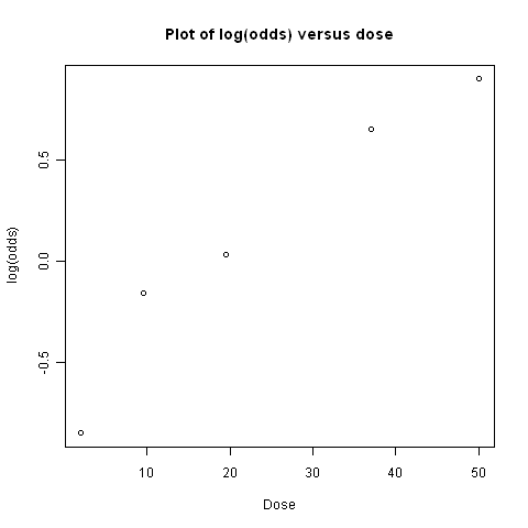
plot(doses,myodds,xlab="Dose",ylab="log(odds)",main="Plot of log(odds) versus dose")
}
We can then use the function doseOddsDiseaseRegression() to test whether the slope of the linear regression line for log(odds) versus dose is significantly different from zero, and also to make a plot of log(odds) versus dose:
> doseOddsDiseaseRegression(mymatrix)
[1] "pvalue for F-test of zero slope = 0.00659217584881777"
The p-value for the test is less than 0.05, so there is evidence that the slope of the linear regression line is significantly different from zero (using a p-value threshold of <0.05 for statistical significance). That is, there seems to be a significant relationship between dose and odds of having the disease given exposure.
Calculating the Sample Size Required for a Randomised Control Trial
A common task in biomedical statistics is to calculate the sample size required, if you want to carry out a randomised control trial with two groups (for example, where one group will take a drug that you want to test, and the other group will take a placebo). You can calculate the sample size required in each group using the following function, “calcSampleSizeForRCT()”, which you will need to copy and paste into R to use:
> calcSampleSizeForRCT <- function(alpha,gamma,piT,piC,p=0)
{
   # p is the estimated of the likely fraction of losses to follow-up
   qalpha <- qnorm(p=1-(alpha/2))
   qgamma <- qnorm(p=gamma)
   pi0 <- (piT + piC)/2
   numerator <- 2 * ((qalpha + qgamma)^2) * pi0 * (1 - pi0)
   denominator <- (piT - piC)^2
   n <- numerator/denominator
   n <- ceiling(n) # round up to the nearest integer
   # adjust for likely losses to folow-up
   n <- n/(1-p)
   n <- ceiling(n) # round up to the nearest integer
   print(paste("Sample size for each trial group = ",n))
}
To use the “calcSampleSizeForRCT()” function, you need to specify the significance level that you want to have, the power that you want to have, the estimated incidence of the disease in the control group (the group taking a placebo), and the estimated incidence of the disease in the treatment group (the group taking the drug). For example, if you want to have a 5% significance level and 90% power, and the estimated incidences of the disease in the control and study groups is 0.20 and 0.15, respectively, then to calculate the required sample size for each group, you would type:
> calcSampleSizeForRCT(alpha=0.05, gamma=0.90, piT=0.15, piC=0.2)
[1] "Sample size for each trial group =  1214"
This tells us that the sample size required in each group is 1214 people, so overall we need 1214*2=2428 people in the randomised control trial.
If we estimate that there are likely to be a certain fraction of people who are lost to follow-up, we can adjust our estimates of the number of people required for the trial. For example, if we estimate that 10% of the people are likely to be lost to follow-up, we can calculate the number of people required for the trial as:
> calcSampleSizeForRCT(alpha=0.05, gamma=0.90, piT=0.15, piC=0.2, p=0.1)
[1] "Sample size for each trial group =  1349"
This tells us that, if 10% of people are likely to be lost to follow-up, we need to have 1349 people in each group in our trial, so 1349*2=2698 people overall.
Calculating the Power of a Randomised Control Trial
If, for practical reasons, you can only have a maximum of a certain number of people in each group of your randomised control trial, then you can calculate the statistical power that your trial will have. You can do this using the following function, “calcPowerForRC()”:
> calcPowerForRCT <- function(alpha,piT,piC,n)
{
   qalpha <- qnorm(p=1-(alpha/2))
   pi0 <- (piT + piC)/2
   denominator <- 2 * pi0 * (1 - pi0)
   fraction <- n/denominator
   qgamma <- (abs(piT - piC) * sqrt(fraction)) - qalpha
   gamma <- pnorm(qgamma)
   print(paste("Power for the randomised controlled trial = ",gamma))
}
For example, to calculate the power of a randomised control trial involving 500 children (250 in the control group and 250 in the treatment group), where the significance level is 0.05, and the estimated incidence of the disease in the control and treatment group is 0.3 and 0.2, respectively, we type:
> calcPowerForRCT(alpha=0.05, piT=0.2, piC=0.3, n=250)
[1] "Power for the randomised controlled trial =  0.73303725668939"
This tells us that the power for the randomised control trial will be 73%.
Making a Forest Plot for a Meta-analysis of Several Different Randomised Control Trials:
If you want to carry out a meta-analysis of several different randomised control trials, it is useful to make a forest plot to display the data. For example, the results of several different randomised control trials may be as follows:
Data for trial 1:
| Disease | Control | |
|---|---|---|
| Exposure | 198 | 728 |
| Unexposed | 128 | 576 |
Data for trial 2:
| Disease | Control | |
|---|---|---|
| Exposure | 96 | 437 |
| Unexposed | 101 | 342 |
Data for trial 3:
| Disease | Control | |
|---|---|---|
| Exposure | 1105 | 4243 |
| Unexposed | 1645 | 6703 |
Data for trial 4:
| Disease | Control | |
|---|---|---|
| Exposure | 741 | 2905 |
| Unexposed | 594 | 2418 |
Data for trial 5:
| Disease | Control | |
|---|---|---|
| Exposure | 264 | 1091 |
| Unexposed | 907 | 3671 |
Data for trial 6:
| Disease | Control | |
|---|---|---|
| Exposure | 105 | 408 |
| Unexposed | 348 | 1248 |
Data for trial 7:
| Disease | Control | |
|---|---|---|
| Exposure | 138 | 431 |
| Unexposed | 436 | 1576 |
We can enter the data into R as follows:
> mymatrix1 <- matrix(c(198,728,128,576),nrow=2,byrow=TRUE)
> mymatrix2 <- matrix(c(96,437,101,342),nrow=2,byrow=TRUE)
> mymatrix3 <- matrix(c(1105,4243,1645,6703),nrow=2,byrow=TRUE)
> mymatrix4 <- matrix(c(741,2905,594,2418),nrow=2,byrow=TRUE)
> mymatrix5 <- matrix(c(264,1091,907,3671),nrow=2,byrow=TRUE)
> mymatrix6 <- matrix(c(105,408,348,1248),nrow=2,byrow=TRUE)
> mymatrix7 <- matrix(c(138,431,436,1576),nrow=2,byrow=TRUE)
> mylist <- list(mymatrix1,mymatrix2,mymatrix3,mymatrix4,mymatrix5,mymatrix6,mymatrix7)
We can then make a forest plot of the data using the following function, “makeForestPlotForRCTs()”, which makes use of the R “rmeta” package (and requires that you have installed the “rmeta” package):
> makeForestPlotForRCTs <- function(mylist, referencerow=2)
{
   require("rmeta")
   numstrata <- length(mylist)
   # make an array "ntrt" of the number of people in the exposed group, in each stratum
   # make an array "nctrl" of the number of people in the unexposed group, in each stratum
   # make an array "ptrt" of the number of people in the exposed group that have the disease,
   # in each stratum
   # make an array "pctrl" of the number of people in the unexposed group that have the disease,
   # in each stratum
   ntrt <- vector()
   nctrl <- vector()
   ptrt <- vector()
   pctrl <- vector()
   if (referencerow == 1) { nonreferencerow <- 2 }
   else                   { nonreferencerow <- 1 }
   for (i in 1:numstrata)
   {
      mymatrix <- mylist[[i]]
      DiseaseUnexposed <- mymatrix[referencerow,1]
      ControlUnexposed <- mymatrix[referencerow,2]
      totUnexposed <- DiseaseUnexposed + ControlUnexposed
      nctrl[i] <- totUnexposed
      pctrl[i] <- DiseaseUnexposed
      DiseaseExposed <- mymatrix[nonreferencerow,1]
      ControlExposed <- mymatrix[nonreferencerow,2]
      totExposed <- DiseaseExposed + ControlExposed
      ntrt[i] <- totExposed
      ptrt[i] <- DiseaseExposed
    }
    names <- as.character(seq(1,numstrata))
    myMH <- meta.MH(ntrt, nctrl, ptrt, pctrl, conf.level=0.95, names=names)
    print(myMH)
    tabletext<-cbind(c("","Study",myMH$names,NA,"Summary"),
       c("Disease","(exposed)",ptrt,NA,NA),
       c("Disease","(unexposed)",pctrl, NA,NA),
       c("","OR",format(exp(myMH$logOR),digits=2),NA,format(exp(myMH$logMH),digits=2)))
    print(tabletext)
    m<- c(NA,NA,myMH$logOR,NA,myMH$logMH)
    l<- m-c(NA,NA,myMH$selogOR,NA,myMH$selogMH)*2
    u<- m+c(NA,NA,myMH$selogOR,NA,myMH$selogMH)*2
    forestplot(tabletext,m,l,u,zero=0,is.summary=c(TRUE,TRUE,rep(FALSE,8),TRUE),
       clip=c(log(0.1),log(2.5)), xlog=TRUE,
       col=meta.colors(box="royalblue",line="darkblue", summary="royalblue"))
}
We can then make a forest plot of the data from the seven different trials by typing:
> makeForestPlotForRCTs(mylist)
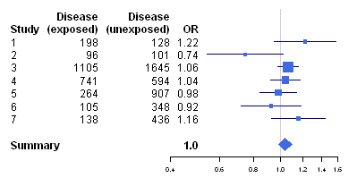
We can use the “calcTaronesTest()” function to perform Tarone’s test (see above), to test whether there is a significant difference between the seven trials in the odds ratio for association between the disease and the exposure:
> calcTaronesTest(mylist)
[1] "Pvalue for Tarone's test = 0.190239054737704"
Here the p-value for Tarone’s test is greater than 0.05, indicating that there is no evidence for a significant difference in the odds ratio between the different strata (between the seven trials, in this example), when a p-value threshold of <0.05 is used for statistical significance.
Links and Further Reading
Some links are included here for further reading.
For a more in-depth introduction to R, a good online tutorial is available on the “Kickstarting R” website, cran.r-project.org/doc/contrib/Lemon-kickstart.
There is another nice (slightly more in-depth) tutorial to R available on the “Introduction to R” website, cran.r-project.org/doc/manuals/R-intro.html.
Robin Beaumont has put some course material on using R for medical statistics on his webpage.
You can find a list of R packages for analysing clinical trial data on the CRAN Clinical Trials Task View.
To learn about biomedical statistics, I would highly recommend the book “Medical statistics” (product code M249/01) by the Open University, available from the Open University Shop.
Acknowledgements
Thank you to Noel O’Boyle for helping in using Sphinx, http://sphinx.pocoo.org, to create this document, and github, https://github.com/, to store different versions of the document as I was writing it, and readthedocs, http://readthedocs.org/, to build and distribute this document.
Many of the examples in this booklet are inspired by examples in the excellent Open University book, “Medical Statistics” (product code M249/01), available from the Open University Shop.
For very helpful comments and suggestions for improvements, I would like to say thank you very much to: Tony Burton, Richard A. Friedman, Duleep Samuel, R.Heberto Ghezzo, David Levine, Lavinia Gordon, Friedrich Leisch, and Phil Spector.
Contact
I will be grateful if you will send me (Avril Coghlan) corrections or suggestions for improvements to my email address alc@sanger.ac.uk
License
The content in this book is licensed under a Creative Commons Attribution 3.0 License.